Python In Excel
Excel's most powerful feature that almost no one uses
In 2024 Microsoft released the Python in Excel feature, yet I have never seen anyone use it - despite it being generally available. So I decided to try it myself, and it’s great. Let me show you how it can be used in daily Structural Engineer work.
And let me be clear: I’m not a fan of Excel for structural calculations, but I can’t escape from reality.
Visualisation
The best use case for me is visualization. Using matplotlib, I can visualize much more than standard built-in charts - shapes, dimensions, colors, finite element meshes, legends, and more.
Soil Profile Example
A lot of the spreadsheets in my private library involve geotechnical calculations, and all of them have a soil profile. Previously it was just a table, but with Python in Excel I can dynamically plot the soil profile.
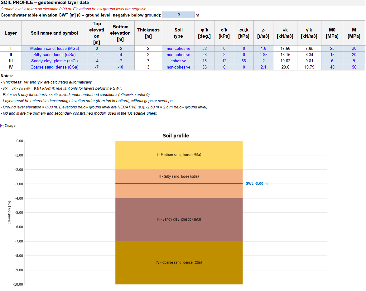
Soil profile plotted dynamically with Python in Excel.
Strip Footing Example
Another real-life example is a spreadsheet for strip footings I wrote a while ago, but it always lacked good visuals, so I hesitated to use it for official printouts. Now I can plot a nice, dynamic figure and include it directly in the final report.
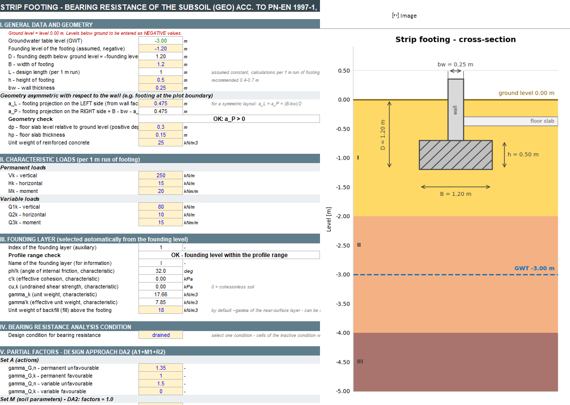
Strip footing geometry plotted with Python in Excel.
Computation
This is serious stuff - you can use pandas, numpy, and scipy, which makes a lot of things possible: matrix math, statistics, and other scientific computation.
The full list of libraries Excel is equipped with can be found in the official library list.
2D Reinforcement for In-Plane Conditions
I want to walk through computing tension reinforcement for in-plane stress, per Eurocode 2 Annex F.
Let’s assume we have FEA results from software that doesn’t support Eurocode 2 shell design, but can export nodes, elements, and corresponding stresses into Excel. Using Python in Excel, we can quickly and cleanly compute the reinforcement ratio for each element.
The standard Eurocode math:
Tensile Forces ($f_{tdx}, f_{tdz}$)
Given stress components $\sigma_{xx}, \sigma_{zz}, \sigma_{xz}$:
Case 1: Full Compression ($\sigma_{xx} < 0$, $\sigma_{zz} \le 0$, and $\sigma_{xx}\sigma_{zz} > \sigma_{xz}^2$)
Case 2: Pure Tensile / Low Compression ($\sigma_{xx} \ge -|\sigma_{xz}|$ and $\sigma_{zz} \ge -|\sigma_{xz}|$)
Case 3: High Compression in X ($\sigma_{zz} \ge \sigma_{xx}$ and $\sigma_{xx} \le -|\sigma_{xz}|$)
Case 4: High Compression in Z ($\sigma_{xx} > \sigma_{zz}$ and $\sigma_{zz} \le -|\sigma_{xz}|$)
Default / Fallback:
Reinforcement Ratios & Areas
Using yield strength $f_{yd}$ and thickness $th$:
Reinforcement Ratios:
Reinforcement Areas:
This is transformed into the following Python code:
import pandas as pd

stress = xl("Stress[#All]", headers=True)
stress = stress[stress["layer"] == "mid"]
for col in ["sxx", "syy", "szz", "sxy", "syz", "szx"]:
    stress[col] = pd.to_numeric(stress[col], errors="coerce")

fyd = 434.8e6
th = 0.2  # Thickness and fy can be a dynamic input


def calculate_rc_ratio(stress_tensor, fyd, th):
    sxx = stress_tensor[0]
    szz = stress_tensor[2]
    sxz = stress_tensor[4]
    if -sxx > 0 and -szz >= 0 and sxx * szz > sxz**2:
        f_tdx = 0
        f_tdz = 0
    elif szz >= sxx and sxx >= -1 * abs(sxz):
        f_tdx = sxx + abs(sxz)
        f_tdz = szz + abs(sxz)
    elif szz >= sxx and -1 * abs(sxz) >= sxx:
        f_tdx = 0
        f_tdz = szz + abs(sxz) ** 2 / sxx
    elif sxx > szz and szz > -1 * abs(sxz):
        f_tdx = sxx + abs(sxz)
        f_tdz = szz + abs(sxz)
    elif sxx > szz and -1 * abs(sxz) >= szz:
        f_tdx = sxx + abs(sxz) ** 2 / szz
        f_tdz = 0
    else:
        f_tdx = 0
        f_tdz = 0
    rc_x = f_tdx / fyd
    rc_z = f_tdz / fyd
    arc_x = rc_x * th
    arc_z = rc_z * th
    return rc_x, rc_z, arc_x, arc_z


out = stress[["element_id", "local_index", "node_id"]].reset_index(drop=True)
res = stress.apply(
    lambda r: calculate_rc_ratio(
        [r["sxx"], r["syy"], r["szz"], r["sxy"], r["szx"], r["syz"]], fyd, th
    ),
    axis=1,
    result_type="expand",
)
res.columns = ["rc_x", "rc_z", "arc_x", "arc_z"]
pd.concat([out, res], axis=1)
The result gets printed into cells, and Python can then be used again for visualisation.
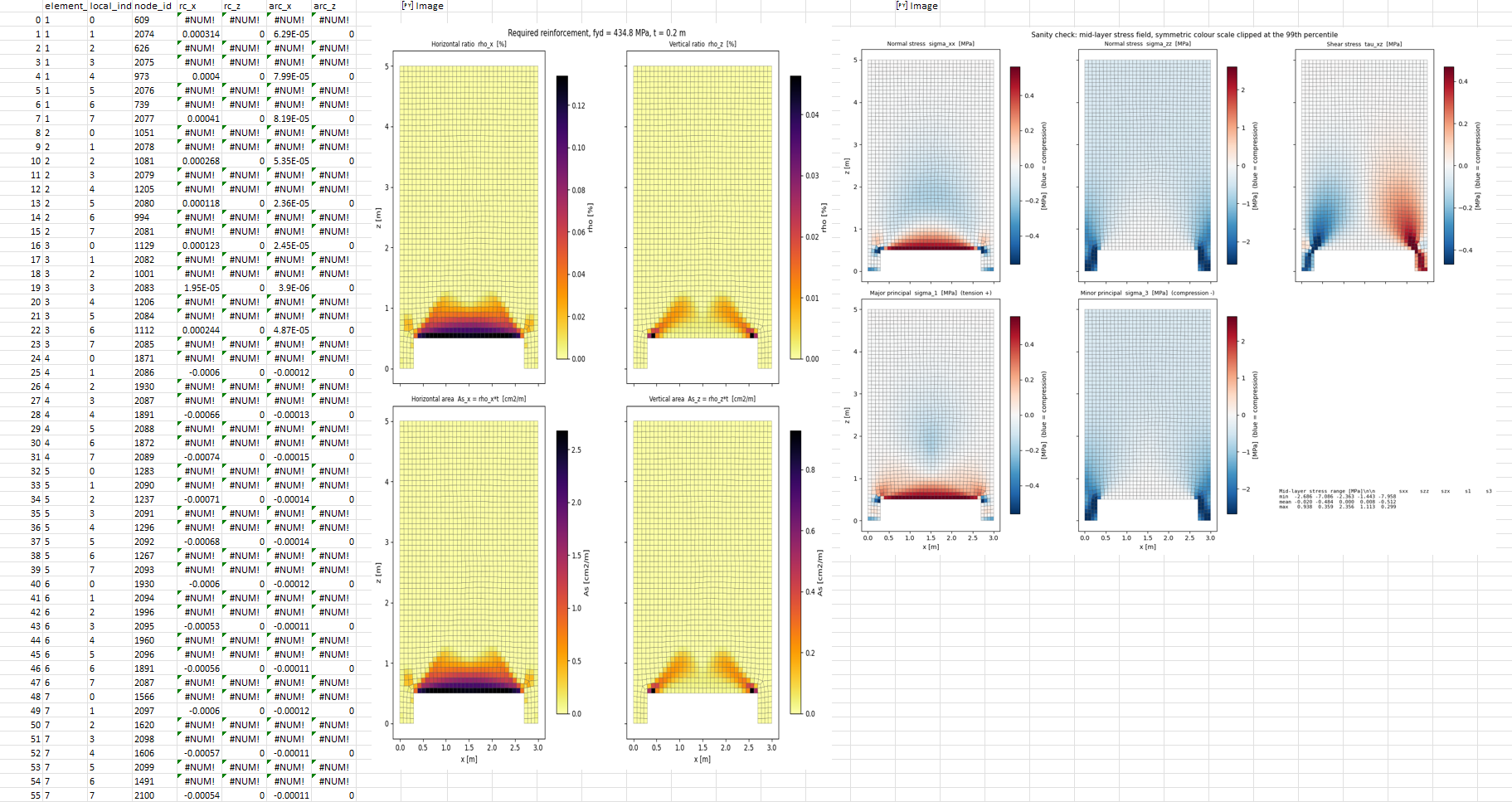
Reinforcement ratio results visualized in Excel via Python.
These are just a few examples from my private library. In a similar manner, I’ve used this for visualization in commercial work as well - for example, in a soil subgrade calculator built from FE data exported from calculation software.
You Don’t Need to Know How to Code
Just ask AI to build the code for you - remember to explicitly mention “Python in Excel” in your prompt.
I’ve tested both Copilot in Excel and Claude in Excel, and both work great. You can also use AI models outside of Excel, but the built-in ones have full access to your data, which saves time.
Why This Is Useful
Not everyone knows Python, and people hesitate to use things that look complicated. The Excel interface helps bridge that gap - you can build small things that make a real difference for your team, and make your reports look good.
How to Start
Go to “Formulas” on the top ribbon and check if you can see the Python tools. If yes, you’re good to go - just prompt an AI. Results go into a cell, preceded by =PY, then use Ctrl+Enter to commit the code into the cell.
Limitations
The solution isn’t perfect. Limitations I’ve found so far:
- Excel has a limit of 8,192 characters per formula, and the code is treated as a formula - so keep code light, avoid unnecessary comments, and use one-liners where possible.
- There are some computation limits; I wouldn’t recommend it for very heavy data, but test the limit yourself.
- Excel sometimes doesn’t cooperate and displays
#CONNECT!- hitting Reset Runtime usually helps. - Error messages are fairly vague, but AI usually handles working through them.
- You’re restricted to the preinstalled libraries - it’s a closed box, with no option to install additional packages or to import/export files outside of the Excel file itself.
See the official documentation for this feature.